Biostatistics & Epidemiology
Study design, descriptive and inferential statistics, hypothesis testing, sensitivity/specificity, odds and relative risk, confidence intervals, bias, confounding, clinical trial methodology, evidence-based medicine principles, and every statistical test, epidemiologic measure, and study design concept across the full scope of medical biostatistics and epidemiology.
01 Overview & Role of Biostatistics
Biostatistics and epidemiology are the quantitative foundations of evidence-based medicine. Biostatistics applies statistical methods to biological, medical, and public health data, while epidemiology is the study of the distribution and determinants of health-related states in populations. Together they provide the framework for designing studies, analyzing data, interpreting medical literature, evaluating diagnostic tests, measuring disease burden, and making clinical and public health decisions grounded in data rather than anecdote.
Every clinical guideline, every drug approval, every screening recommendation, and every risk estimate a physician communicates to a patient rests on biostatistical and epidemiologic reasoning. A clinician who cannot interpret a confidence interval, compute a likelihood ratio, or distinguish a cohort from a case-control study cannot critically evaluate the evidence base of modern medicine.
Core Domains
| Domain | Focus |
|---|---|
| Descriptive statistics | Summarizing and presenting data (mean, median, SD, graphs) |
| Inferential statistics | Drawing conclusions about populations from samples (hypothesis testing, CIs) |
| Epidemiology | Disease frequency, determinants, and distribution in populations |
| Study design | Observational and experimental methods for investigating health questions |
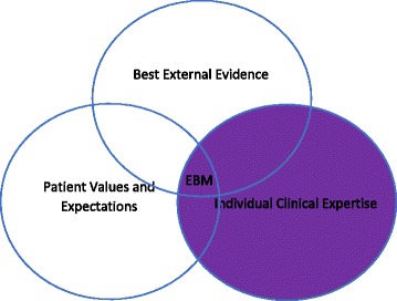
| Evidence-based medicine | Integration of best research evidence with clinical expertise and patient values |
| Clinical epidemiology | Applying epidemiologic methods to clinical decision-making |
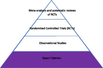
Evidence-Based Medicine Hierarchy
Not all evidence is created equal. The traditional hierarchy of evidence, from strongest to weakest: systematic reviews and meta-analyses of RCTs → individual randomized controlled trials → cohort studies → case-control studies → cross-sectional studies → case series and case reports → expert opinion and bench research. Higher-level evidence generally has better control of bias and confounding, but the best study design depends on the clinical question.
Historical Context
Modern biostatistics traces its origins to the 17th century with John Graunt's analysis of London bills of mortality, but the discipline was transformed by the work of Pierre-Charles-Alexandre Louis in 19th century Paris, who used the "numerical method" to disprove the benefit of bloodletting in pneumonia. The 20th century brought Ronald Fisher's foundational work on statistical inference, the first modern randomized controlled trial (streptomycin for tuberculosis in 1948 by Bradford Hill), and the landmark Framingham Heart Study (1948), which introduced the idea of "risk factors" for cardiovascular disease and established cohort methodology as a mainstay of chronic disease epidemiology.
The discipline was further shaped by major epidemiologic achievements: John Snow tracing the 1854 London cholera outbreak to the Broad Street pump, Doll and Hill establishing the smoking-lung cancer link in the 1950s, the publication of the first Cochrane systematic reviews in the 1990s, and the emergence of large genome-wide association studies (GWAS) in the 2000s. Each of these milestones required new biostatistical methods that now form part of standard practice.
Biostatistics appears on every step of the USMLE and on every clinical shelf and board exam. More importantly, it is tested implicitly every day at the bedside: interpreting a troponin level, explaining a Gail model risk, quoting a number needed to treat, deciding whether a screening test is warranted. Fluency in these concepts is not optional — it is a core clinical skill.
02 Core Terminology & Definitions
A shared vocabulary is essential for reading the medical literature. Misinterpretation of statistical terms is one of the most common sources of error in clinical reasoning.
Foundational Terms
| Term | Definition |
|---|---|
| Population | The entire group of interest (e.g., all adults with hypertension) |
| Sample | Subset of the population actually studied |
| Parameter | Numeric characteristic of a population (usually unknown, e.g., μ) |
| Statistic | Numeric characteristic calculated from a sample (e.g., sample mean x̄) |
| Null hypothesis (H0) | Statement of no effect or no difference |
| Alternative hypothesis (H1) | Statement that there is an effect or difference |
| Incidence | New cases per population at risk over time |
| Prevalence | Existing cases at a point in time / population |
| Risk | Probability of an event occurring within a defined time period |
| Odds | Probability of event / probability of no event |
| Exposure | Factor hypothesized to influence outcome |
| Outcome | Event or condition being measured |
| Confidence interval | Range of plausible values for a parameter at specified confidence level |
| p-value | Probability of observing data as extreme as the result, assuming H0 true |
| Effect size | Magnitude of the observed effect (clinical importance) |
| Validity | Accuracy; degree to which a measurement reflects truth |
| Reliability | Reproducibility; consistency of measurement |
| Precision | Degree of random error; narrow CI indicates high precision |
| Accuracy | Degree to which measurement approximates the true value |
A broken bathroom scale that always reads 5 pounds too high is reliable (consistent) but not valid (inaccurate). A scale that gives wildly different readings on repeated weighings is neither reliable nor valid. The goal in medical measurement is both — reproducible and accurate.
Descriptive vs Analytic Epidemiology
Descriptive epidemiology answers "who, what, when, where" — characterizing disease distribution by person, place, and time. It generates hypotheses. Analytic epidemiology answers "why and how" by formally testing associations between exposures and outcomes. Most clinical research involves analytic epidemiology, but descriptive work remains essential for surveillance, outbreak detection, and public health planning.
Statistical Symbols
| Symbol | Meaning |
|---|---|
| μ (mu) | Population mean |
| x̄ (x-bar) | Sample mean |
| σ (sigma) | Population standard deviation |
| s | Sample standard deviation |
| σ² / s² | Variance |
| n / N | Sample size / population size |
| α (alpha) | Type I error rate (significance level) |
| β (beta) | Type II error rate |
| 1 − β | Statistical power |
03 Types of Data & Variables
The type of variable dictates which descriptive statistics and which statistical tests are appropriate. Misclassification of variable type is a common error that leads to choosing the wrong statistical test.
Variable Classification
| Type | Subtype | Description | Examples |
|---|---|---|---|
| Categorical (qualitative) | Nominal | Unordered categories | Blood type, gender, race |
| Ordinal | Ordered categories, unequal intervals | Pain scale, NYHA class, tumor stage | |
| Numerical (quantitative) | Discrete | Countable integers | Number of children, hospital admissions |
| Continuous | Measurable, infinite values | Blood pressure, weight, serum sodium |
Continuous variables are further subdivided into interval data (meaningful intervals, no true zero; e.g., Celsius temperature) and ratio data (meaningful intervals with a true zero; e.g., weight, Kelvin temperature). Ratio data permits statements about multiplication ("twice as heavy"), whereas interval data does not.
Independent vs Dependent Variables
The independent variable (predictor, exposure) is the factor manipulated or observed as the presumed cause. The dependent variable (outcome, response) is the variable measured as the presumed effect. In a study of smoking and lung cancer, smoking status is the independent variable and lung cancer incidence is the dependent variable.
Data Transformation
Skewed continuous data can sometimes be transformed to approximate normality, allowing the use of parametric tests. Common transformations include the logarithmic transformation (for right-skewed data like serum triglycerides, cytokine concentrations, or hospital length of stay), the square root transformation (for count data or mildly skewed data), and the reciprocal transformation (for highly skewed data). Transformation should be pre-specified in the analysis plan whenever possible to avoid data dredging.
Dichotomization Pitfalls
Converting continuous variables to binary categories (e.g., defining hypertension as BP ≥ 140/90) is common but statistically inefficient. Dichotomization reduces statistical power, assumes a sharp biological threshold that rarely exists, and discards clinically relevant information. Where possible, continuous variables should be analyzed as continuous. Clinical cutoffs are useful for decision-making but should not drive statistical analysis.
04 Measures of Central Tendency
Measures of central tendency describe the "typical" or "center" value of a dataset. The three classical measures are the mean, median, and mode, each with different strengths depending on data distribution.
Mean, Median, Mode
| Measure | Definition | Best Used For | Sensitive to Outliers? |
|---|---|---|---|
| Mean (μ, x̄) | Sum of values ÷ n | Normally distributed continuous data | Yes (strongly) |
| Median | Middle value when sorted (50th percentile) | Skewed data, ordinal data | No (robust) |
| Mode | Most frequently occurring value | Categorical/nominal data; bimodal distributions | No |
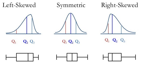
Relationship in Skewed Distributions
The relative position of mean, median, and mode reveals distribution shape:
- Symmetric (normal): Mean = Median = Mode
- Positive (right) skew: Mean > Median > Mode (tail on right; e.g., income, length of hospital stay)
- Negative (left) skew: Mean < Median < Mode (tail on left; e.g., age at death, test scores with ceiling effects)
Weighted Mean & Geometric Mean
When observations carry different weights (e.g., pooled studies in meta-analysis or laboratories contributing different sample sizes), the weighted mean gives disproportionate influence to larger or more reliable data points. The geometric mean — the nth root of the product of n values — is appropriate for log-normally distributed data like antibody titers, viral loads, or drug concentrations, where ratios matter more than differences. The harmonic mean is used for averaging rates (e.g., F1 score combining precision and recall).
Choosing a Measure
For symmetric continuous data, the mean is most efficient and commonly reported. For skewed data (income, LOS, cost), report the median with IQR. For categorical or nominal data, report the mode or percentages. When in doubt, report multiple measures and the distribution shape, and let readers judge.
05 Measures of Dispersion
Measures of dispersion quantify how spread out data are around the center. Two datasets can share the same mean but differ dramatically in variability, which matters enormously for clinical interpretation.
Common Measures of Spread
| Measure | Formula / Definition | Comment |
|---|---|---|
| Range | Maximum − minimum | Very sensitive to outliers; ignores distribution |
| Variance (s²) | Σ(xi − x̄)² ÷ (n−1) | Average squared deviation from the mean |
| Standard deviation (s) | √variance | Same units as data; most common dispersion measure |
| Interquartile range (IQR) | Q3 − Q1 (75th − 25th percentile) | Robust to outliers; paired with median |
| Standard error (SE) | s / √n | SD of the sampling distribution of the mean |
| Coefficient of variation | (s / x̄) × 100% | Relative variability; allows comparison across units |
Standard deviation describes variability among individual observations in the sample. Standard error describes variability of the sample mean if the study were repeated many times. SE is always smaller than SD (SE = SD/√n). Use SD to describe data; use SE to construct confidence intervals around estimates. Papers that report SE instead of SD to make spread look smaller are committing a common deception.
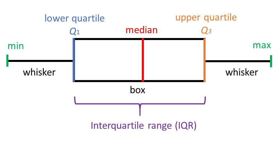
Percentiles & Quartiles
The nth percentile is the value below which n% of observations fall. The median is the 50th percentile. Q1 (25th), Q2 (50th), and Q3 (75th) are the quartiles, and the IQR (Q3 − Q1) contains the middle 50% of data. Box plots graphically display the median, IQR, and outliers.
06 Distributions & Normality
The shape of a data distribution determines which statistical methods are valid. Most inferential statistical tests assume specific distributional properties, and violating these assumptions can produce misleading results.
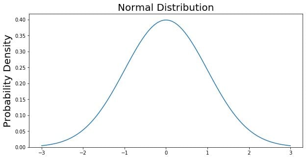
The Normal (Gaussian) Distribution
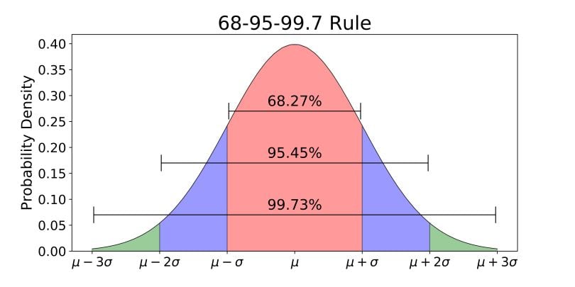
The normal distribution is a symmetric, bell-shaped curve characterized by its mean and standard deviation. Its critical properties underpin most parametric statistics:
- Symmetric about the mean; mean = median = mode
- 68% of data falls within ±1 SD of the mean
- 95% of data falls within ±1.96 SD (≈ 2 SD) of the mean
- 99.7% of data falls within ±3 SD of the mean
- Total area under the curve = 1
Other Distribution Shapes
| Distribution | Description | Clinical Example |
|---|---|---|
| Normal | Symmetric, bell-shaped | Adult height, hemoglobin in healthy adults |
| Positive (right) skew | Long right tail | Hospital length of stay, serum triglycerides |
| Negative (left) skew | Long left tail | Age at death in developed nations |
| Bimodal | Two peaks | Hodgkin lymphoma age (peaks at 20s and 60s) |
| Uniform | Flat, all values equally likely | Random number generator output |
| Poisson | Discrete count of rare events | ED visits per hour, radioactive decay counts |
| Binomial | Two discrete outcomes | Coin flips, success/failure trials |
Z-Scores & Standardization
A z-score expresses how many standard deviations a value lies from the mean: z = (x − μ) / σ. Z-scores allow comparison across variables measured on different scales. A z of +2 means the value is 2 SD above the mean (> 97.5th percentile in a normal distribution).
Assessing Normality
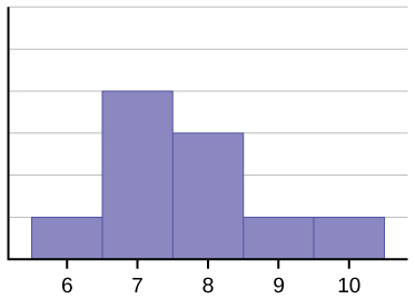
Before applying parametric tests, researchers should assess whether data are approximately normal. Methods include:
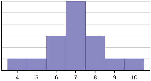
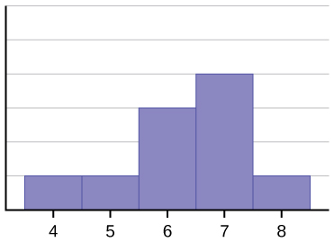
- Visual inspection: Histograms, Q-Q plots, and box plots reveal skewness, bimodality, and outliers
- Formal tests: Shapiro-Wilk test (preferred for small samples), Kolmogorov-Smirnov test, Anderson-Darling test. With large samples (n > 100), these tests become overly sensitive and may reject normality for minor deviations that do not affect inference.
- Skewness & kurtosis values: Skewness near 0 and kurtosis near 3 suggest normality
07 Probability & Sampling
Probability is the mathematical language of uncertainty and the foundation of inferential statistics. Sampling methods determine whether study results can be generalized to the target population.
Rules of Probability
| Rule | Formula | Application |
|---|---|---|
| Range | 0 ≤ P(A) ≤ 1 | Probabilities are always between 0 and 1 |
| Complement | P(not A) = 1 − P(A) | P(disease absent) = 1 − P(disease) |
| Addition (mutually exclusive) | P(A or B) = P(A) + P(B) | Dying from disease A or B (can't be both) |
| Addition (non-exclusive) | P(A or B) = P(A) + P(B) − P(A and B) | Having HTN or DM (some have both) |
| Multiplication (independent) | P(A and B) = P(A) × P(B) | Two independent test results |
| Conditional | P(A|B) = P(A and B) / P(B) | P(disease | positive test) |
Sampling Methods
| Method | Description | Use |
|---|---|---|
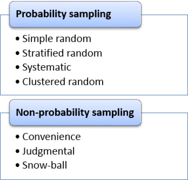
| Simple random | Every individual has equal chance of selection | Gold standard; requires sampling frame |
| Stratified | Random samples within subgroups (strata) | Ensures representation of minority subgroups |
| Cluster | Randomly select groups (clusters), then sample within | Geographically dispersed populations |
| Systematic | Every kth individual after a random start | Simple but vulnerable to periodicity bias |
| Convenience | Whoever is easily accessible | High risk of selection bias; avoid when possible |
| Snowball | Participants recruit other participants | Hard-to-reach populations (IV drug users, MSM) |
08 Central Limit Theorem & Standard Error
The central limit theorem (CLT) is the single most important result in statistics. It provides the theoretical foundation that allows statisticians to make inferences about population parameters from sample data even when the underlying population is not normally distributed.
As sample size n increases, the sampling distribution of the sample mean approaches a normal distribution regardless of the shape of the underlying population distribution, with mean μ and standard deviation σ/√n (the standard error). In practice, n ≥ 30 is usually sufficient for the CLT to apply.
Implications
The CLT means that even if individual patient blood pressures are skewed, the distribution of sample means from repeated studies will be approximately normal. This allows use of normal-based inference (z-tests, t-tests, confidence intervals) for most research questions involving means, as long as the sample is reasonably large.
Standard Error of the Mean
The standard error of the mean (SEM) quantifies the precision of the sample mean as an estimate of the population mean: SEM = s / √n. Doubling the sample size reduces SE by a factor of √2, not 2 — precision improves but with diminishing returns. Quadrupling n is required to halve the SE.
09 Confidence Intervals
A confidence interval (CI) provides a range of plausible values for a population parameter based on sample data. CIs convey both the point estimate and its precision, and are generally preferred over p-values alone for reporting results.
Interpretation
A 95% confidence interval means that if the study were repeated many times, 95% of the constructed intervals would contain the true population parameter. It does not mean there is a 95% probability the true value lies in this particular interval — a common but incorrect interpretation. The parameter is fixed; the interval varies across samples.
Formula for 95% CI of a Mean
95% CI = x̄ ± 1.96 × (SE)
For 99% CI, multiply SE by 2.58. For 90% CI, multiply by 1.645. Wider intervals correspond to higher confidence at the cost of precision.
Width Determinants
| Factor | Effect on CI Width |
|---|---|
| Larger sample size (n) | Narrower CI (more precise) |
| Higher confidence level (99% vs 95%) | Wider CI |
| Greater variability (SD) | Wider CI |
CIs for Other Parameters
| Parameter | 95% CI Formula |
|---|---|
| Mean | x̄ ± 1.96 × (s/√n) |
| Proportion (large n) | p ± 1.96 × √[p(1−p)/n] |
| Difference in means | (x̄1 − x̄2) ± 1.96 × SEdiff |
| Relative risk | Computed on log scale, then exponentiated |
| Odds ratio | Computed on log scale, then exponentiated |
CIs & Statistical Significance
- For means: if the 95% CI for the difference does not cross zero, the result is statistically significant at α = 0.05
- For ratios (RR, OR, HR): if the 95% CI does not cross 1.0, the result is statistically significant
A narrow CI can show statistical significance with trivial clinical impact, while a wide CI may be consistent with both meaningful benefit and harm. A blood pressure drug showing a 0.5 mmHg reduction with 95% CI (0.2–0.8) is statistically significant but clinically worthless. Always evaluate both the magnitude of effect and its precision.
10 Hypothesis Testing & p-Values
Hypothesis testing is the formal framework for deciding whether observed data provide enough evidence to reject a null hypothesis in favor of an alternative. It produces the ubiquitous but frequently misinterpreted p-value.
Steps in Hypothesis Testing
- State the null (H0) and alternative (H1) hypotheses
- Choose the significance level (α), typically 0.05
- Select the appropriate statistical test based on data type and study design
- Calculate the test statistic and corresponding p-value
- Compare p to α: if p < α, reject H0; if p ≥ α, fail to reject H0
- Interpret clinically
p-Value Definition
The p-value is the probability of observing data as extreme (or more extreme) than those actually observed, assuming the null hypothesis is true. A small p-value means the observed data would be unlikely under H0, providing evidence against H0.
A p-value is NOT the probability that the null hypothesis is true. It is NOT the probability the result occurred by chance. It does NOT measure effect size or clinical importance. A statistically significant result (p < 0.05) does not prove the alternative hypothesis. These misinterpretations are so pervasive the American Statistical Association issued a 2016 statement warning against them.
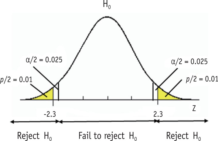
One-Tailed vs Two-Tailed Tests
A two-tailed test examines whether an effect exists in either direction (H1: μ ≠ μ0) and is the default in medical research. A one-tailed test looks only for an effect in a pre-specified direction (H1: μ > μ0) and is justified only when an effect in the opposite direction is either impossible or clinically irrelevant. One-tailed testing doubles the power (halves the p-value) but is considered suspect when chosen post-hoc.
11 Type I, Type II Errors & Power
Statistical inference can go wrong in two ways: rejecting a true null hypothesis (Type I error) or failing to reject a false null hypothesis (Type II error). Understanding these errors is essential for designing studies and interpreting results.
Error Matrix
| H0 True (no effect) | H0 False (effect exists) | |
|---|---|---|
| Reject H0 | Type I error (α) — "false positive" | Correct (power = 1−β) |
| Fail to reject H0 | Correct | Type II error (β) — "false negative" |
Key Definitions
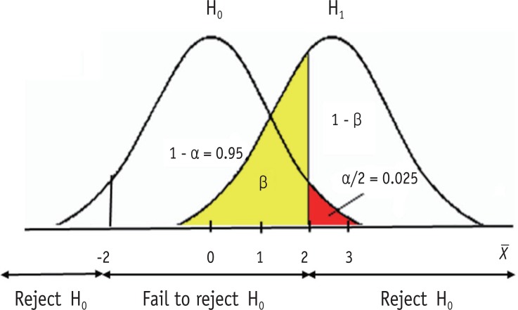
- Type I error (α): Rejecting H0 when it is true. Conventionally set at 0.05, meaning 5% false positive rate.
- Type II error (β): Failing to reject H0 when it is false. Conventionally 0.10–0.20.
- Power (1 − β): Probability of correctly detecting a true effect. Studies are typically designed for 80–90% power.
Determinants of Statistical Power
| Factor | Effect on Power |
|---|---|
| Larger sample size (n) | ↑ Power |
| Larger effect size | ↑ Power |
| Smaller variability (SD) | ↑ Power |
| Higher α level (e.g., 0.10 vs 0.05) | ↑ Power |
| One-tailed vs two-tailed test | ↑ Power (one-tailed) |
Sample size calculations require pre-specifying the effect size of interest, variability (SD), desired power (usually 0.80), and alpha (usually 0.05). Underpowered studies frequently produce false-negative conclusions ("no difference") when real differences exist. A "negative" trial is uninformative without an adequate power calculation.
Multiple Comparisons Problem
When many hypothesis tests are performed in a single study, the probability of at least one false positive rises sharply. Testing 20 independent hypotheses at α = 0.05 yields a 64% probability of at least one false positive under the null. Corrections include:
- Bonferroni correction: Divide α by the number of tests (conservative)
- Holm-Bonferroni: Sequential version, less conservative than Bonferroni
- Benjamini-Hochberg: Controls the false discovery rate (FDR) rather than the family-wise error rate
- Pre-specification of primary and secondary endpoints to limit exploratory analyses
12 Parametric Tests (t-test, ANOVA, Regression)
Parametric tests assume that data follow a known distribution (usually normal) and compare means or other parameters. They are more powerful than non-parametric alternatives when assumptions are met.
t-Tests
| Test | Use | Example |
|---|---|---|
| One-sample t-test | Compare sample mean to a known population mean | Is average BP in clinic different from national average? |
| Independent (unpaired) t-test | Compare means of two independent groups | BP in treatment vs placebo arms |
| Paired t-test | Compare two measurements in same subjects | BP before and after drug in same patients |
Assumptions: continuous outcome, approximately normal distribution, independent observations (except paired), and roughly equal variances (for independent t-test).
ANOVA (Analysis of Variance)
ANOVA extends the t-test to compare means across three or more groups. A one-way ANOVA tests one grouping variable; two-way ANOVA tests two factors simultaneously and can detect interaction effects. The overall F-test indicates whether any groups differ; post-hoc tests (Tukey, Bonferroni) identify which specific groups differ.
| Design | Test |
|---|---|
| 2 independent groups | Independent t-test |
| ≥3 independent groups | One-way ANOVA |
| 2 related measurements | Paired t-test |
| ≥3 related measurements | Repeated-measures ANOVA |
Linear Regression
Linear regression models the relationship between a continuous outcome and one or more predictors: Y = β0 + β1X1 + ... + ε. Simple linear regression uses one predictor; multiple linear regression uses several. The coefficient β1 represents the average change in Y for a one-unit change in X1, adjusting for other variables. R² quantifies the proportion of variance in Y explained by the model.
Assumptions of Linear Regression
- Linearity: The relationship between predictor and outcome is linear
- Independence: Residuals are independent of each other
- Homoscedasticity: Constant variance of residuals across predictor values
- Normality of residuals: Residuals are approximately normally distributed
- No multicollinearity: Predictor variables are not highly correlated with each other
Violations can be detected with residual plots, Q-Q plots, and variance inflation factors (VIF). VIF > 5–10 suggests problematic multicollinearity that may require dropping or combining predictors.
ANCOVA
Analysis of covariance (ANCOVA) combines ANOVA with regression by comparing group means while adjusting for one or more continuous covariates. It is commonly used in RCTs to adjust outcomes for baseline values, increasing precision compared to unadjusted analysis.
13 Non-Parametric Tests (Chi-Square, Mann-Whitney)
Non-parametric tests make fewer assumptions about the underlying distribution. They are appropriate for ordinal data, small samples, or continuous data that is clearly non-normal and cannot be transformed.
Tests for Categorical Data
| Test | Use | Requirements |
|---|---|---|
| Chi-square (χ²) test | Compare proportions across ≥2 groups | Expected cell counts ≥5 in ≥80% of cells |
| Fisher exact test | Compare proportions in 2×2 tables with small samples | Any expected count <5 |
| McNemar test | Paired binary outcomes (before/after same subject) | Matched pairs |
| Cochran-Mantel-Haenszel | Adjust 2×2 tables for confounder strata | Stratified analysis |
Tests for Continuous/Ordinal Data
| Non-Parametric Test | Parametric Equivalent | Use |
|---|---|---|
| Mann-Whitney U (Wilcoxon rank-sum) | Independent t-test | Compare 2 independent groups on ordinal/skewed data |
| Wilcoxon signed-rank | Paired t-test | Compare paired ordinal/skewed data |
| Kruskal-Wallis | One-way ANOVA | Compare ≥3 independent groups |
| Friedman test | Repeated-measures ANOVA | Compare ≥3 related measurements |
| Spearman correlation | Pearson correlation | Rank-based correlation |
14 Survival Analysis & Cox Regression
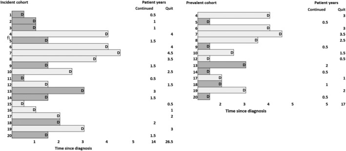
Survival analysis handles time-to-event data, including the challenge of censoring — subjects whose event has not occurred by study end or who are lost to follow-up. It is essential in oncology, cardiology, and transplant medicine.
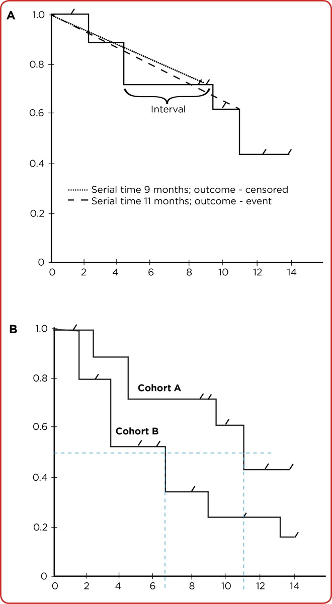
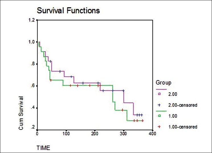
Kaplan-Meier Analysis
The Kaplan-Meier method estimates the survival function — the probability of surviving past time t — and produces the familiar stepwise survival curve. At each event time, the survival probability drops by the fraction of subjects experiencing the event. Censored subjects appear as tick marks and contribute data until censoring.
Log-Rank Test
The log-rank test compares two or more Kaplan-Meier survival curves under the null hypothesis that they are identical. It is the most common test for comparing survival between treatment arms in RCTs.
Cox Proportional Hazards Regression
Cox regression models the hazard ratio (HR) — the instantaneous risk of the event in one group relative to another — while adjusting for covariates. HR = 1 means no difference; HR > 1 means higher hazard; HR < 1 means lower hazard. The key assumption is that hazards are proportional over time (constant HR).
| Method | Purpose |
|---|---|
| Kaplan-Meier curve | Visual display of survival over time |
| Median survival | Time at which 50% of subjects have experienced event |
| Log-rank test | Compare survival between groups (unadjusted) |
| Cox proportional hazards | Adjusted hazard ratios with covariates |
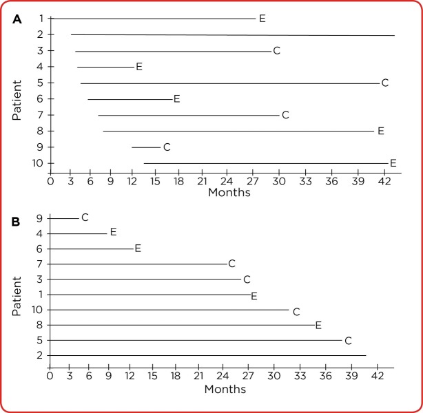
Censoring
Censoring occurs when a subject's event time is not observed — because the study ended, the subject was lost to follow-up, or died from an unrelated cause. Right censoring (the most common type) means the event, if it occurs, will occur after the last observed time. Survival analysis methods assume that censoring is non-informative — that censored subjects have the same underlying risk as those who remain in the study. Violations of this assumption (e.g., sicker patients dropping out) bias the estimates.
Competing Risks
When subjects can experience multiple mutually exclusive outcomes (e.g., death from cancer vs death from heart disease), standard Kaplan-Meier methods overestimate the probability of the outcome of interest. Competing risk methods such as the cumulative incidence function (CIF) and Fine-Gray regression properly account for these alternative events.
15 Correlation & Logistic Regression
Correlation Coefficients
Correlation measures the strength and direction of association between two variables. It does not imply causation.
- Pearson's r: Linear correlation between two continuous, normally distributed variables. Range: −1 to +1.
- Spearman's ρ: Rank-based correlation for ordinal or non-normal continuous data.
- r = 0: no linear relationship; r = ±1: perfect linear relationship
- |r| < 0.3: weak; 0.3–0.7: moderate; > 0.7: strong
Ice cream sales correlate with drownings, but ice cream does not cause drowning; both are driven by summer weather. Before inferring causation, ask whether a third variable (confounder) could explain the association, whether the direction is right (reverse causation), and whether chance or bias might account for it.
Intraclass Correlation & Kappa
When evaluating agreement between observers or methods, different measures apply depending on data type. For categorical data, Cohen's kappa (κ) adjusts observed agreement for chance agreement: κ < 0.2 is slight, 0.2–0.4 fair, 0.4–0.6 moderate, 0.6–0.8 substantial, 0.8–1.0 almost perfect. For continuous data, the intraclass correlation coefficient (ICC) measures reliability between raters. Bland-Altman plots visualize agreement between two measurement methods.
Logistic Regression
Logistic regression is used when the outcome is binary (yes/no, dead/alive, disease/no disease). It models the log-odds of the outcome as a linear function of predictors: ln(p/(1−p)) = β0 + β1X1 + .... Coefficients exponentiated (eβ) give adjusted odds ratios, allowing simultaneous adjustment for multiple confounders.
| Outcome Type | Regression Model |
|---|---|
| Continuous | Linear regression |
| Binary | Logistic regression |
| Time-to-event (with censoring) | Cox proportional hazards |
| Count | Poisson / negative binomial regression |
| Ordinal | Ordinal logistic regression |
16 Sensitivity, Specificity, PPV & NPV
Evaluating diagnostic tests requires understanding their intrinsic properties (sensitivity, specificity) and how those properties translate into clinical predictive values given disease prevalence.
The 2×2 Diagnostic Table
| Disease + | Disease − | Total | |
|---|---|---|---|
| Test + | True Positive (TP) | False Positive (FP) | TP + FP |
| Test − | False Negative (FN) | True Negative (TN) | FN + TN |
| Total | TP + FN | FP + TN | N |
Core Definitions
| Measure | Formula | Interpretation |
|---|---|---|
| Sensitivity (SN) | TP / (TP + FN) | Proportion of diseased correctly identified |
| Specificity (SP) | TN / (TN + FP) | Proportion of healthy correctly identified |
| Positive Predictive Value | TP / (TP + FP) | P(disease | positive test) |
| Negative Predictive Value | TN / (TN + FN) | P(no disease | negative test) |
| Accuracy | (TP + TN) / N | Overall correct classification rate |
| Prevalence | (TP + FN) / N | Proportion with disease in population |
SnNOut: A highly Sensitive test with a Negative result rules OUT disease (few false negatives). Use sensitive tests for screening.
SpPIn: A highly Specific test with a Positive result rules IN disease (few false positives). Use specific tests for confirmation.
Prevalence Dependence of PPV and NPV
Sensitivity and specificity are intrinsic test properties (do not vary with prevalence). PPV and NPV depend heavily on disease prevalence. As prevalence increases, PPV rises and NPV falls. This explains why a highly specific screening test produces many false positives when used in low-prevalence populations (e.g., mammography in 30-year-olds).
Spectrum Bias
The sensitivity and specificity of a test can appear different in different populations due to spectrum bias — the phenomenon that test performance depends on the distribution of disease severity in the study population. A cardiac biomarker tested in patients with obvious STEMI will show higher sensitivity than when tested in patients with ambiguous chest pain. Clinicians should interpret published test characteristics in light of the spectrum of patients studied, not their own clinic.
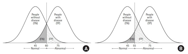
Trade-Off Between Sensitivity and Specificity
For any continuous diagnostic test, lowering the cutoff increases sensitivity at the expense of specificity and vice versa. The ROC curve visualizes this trade-off. Choosing the cutoff requires weighing the relative costs of false positives and false negatives, which depend on disease severity, treatment risks, and downstream workups.
17 Likelihood Ratios & ROC Curves
Likelihood Ratios
Likelihood ratios combine sensitivity and specificity into a single number that quantifies how much a test result changes the probability of disease. Unlike PPV/NPV, LRs are independent of prevalence.
- Positive LR (LR+) = SN / (1 − SP) — how much more likely a positive result occurs in diseased vs healthy
- Negative LR (LR−) = (1 − SN) / SP — how much more likely a negative result occurs in diseased vs healthy
| LR+ | Impact on Probability |
|---|---|
| > 10 | Large increase (often diagnostic) |
| 5–10 | Moderate increase |
| 2–5 | Small increase |
| 1–2 | Minimal; rarely clinically useful |
| 1 | No change (worthless test) |
| LR− | Impact on Probability |
|---|---|
| < 0.1 | Large decrease (often rules out) |
| 0.1–0.2 | Moderate decrease |
| 0.2–0.5 | Small decrease |
| 0.5–1 | Minimal |
Probability-to-Odds Conversion
| Probability | Odds |
|---|---|
| 0.10 | 1:9 (0.11) |
| 0.25 | 1:3 (0.33) |
| 0.50 | 1:1 (1.00) |
| 0.75 | 3:1 (3.00) |
| 0.90 | 9:1 (9.00) |
Conversion: odds = p / (1 − p) and p = odds / (1 + odds). Knowing the relationship is essential for applying Bayes theorem in the odds form.
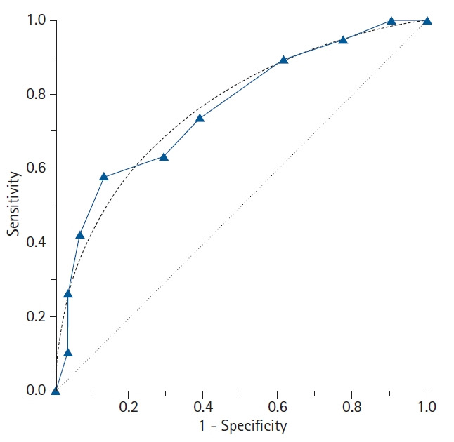
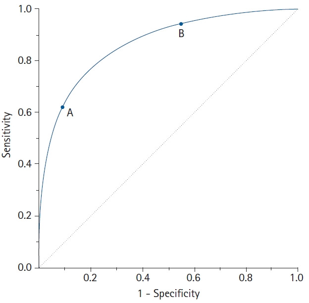
ROC Curves & AUC
A Receiver Operating Characteristic (ROC) curve plots sensitivity (true positive rate) against 1 − specificity (false positive rate) across all possible cutoff values. The area under the curve (AUC) measures overall test discrimination:
| AUC | Discrimination |
|---|---|
| 1.0 | Perfect |
| 0.9–1.0 | Excellent |
| 0.8–0.9 | Good |
| 0.7–0.8 | Fair |
| 0.6–0.7 | Poor |
| 0.5 | No better than chance |
18 Bayes Theorem & Pre/Post-Test Probability
Bayes theorem formalizes how prior knowledge (pre-test probability) combines with new evidence (test results) to update the probability of disease (post-test probability). It is the mathematical foundation of clinical diagnostic reasoning.
The Theorem
P(Disease | Test+) = P(Test+ | Disease) × P(Disease) / P(Test+)
Clinical Form Using Odds and LRs
Post-test odds = Pre-test odds × LR
- Estimate pre-test probability of disease (from prevalence, history, exam)
- Convert probability to odds: odds = p / (1 − p)
- Multiply by LR for the observed test result
- Convert back to probability: p = odds / (1 + odds)
Example
A patient with chest pain has a 30% pre-test probability of acute coronary syndrome. Troponin is positive with an LR+ of 25. Pre-test odds = 0.30/0.70 = 0.43. Post-test odds = 0.43 × 25 = 10.7. Post-test probability = 10.7/11.7 = 91%. Diagnosis essentially confirmed.
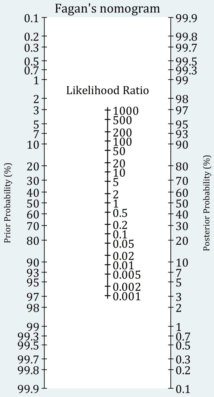
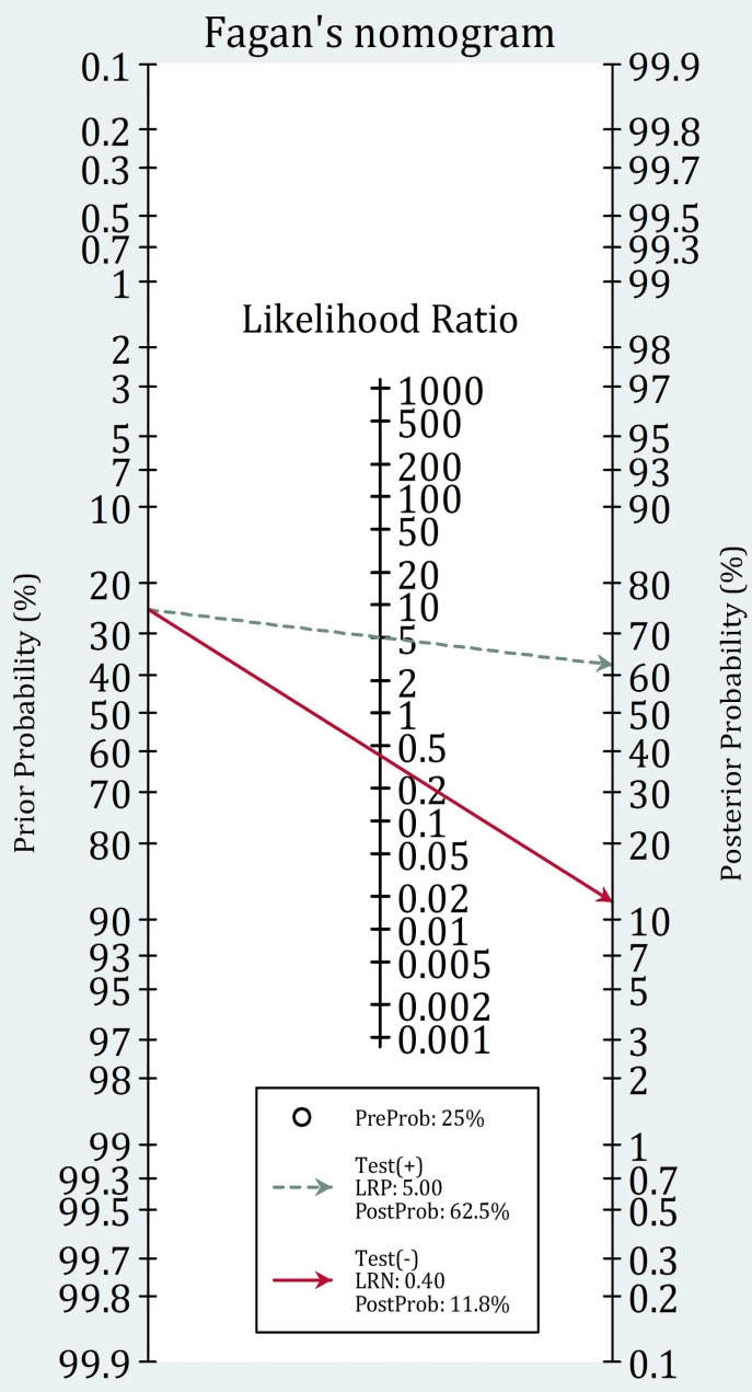
Fagan Nomogram
The Fagan nomogram is a graphical tool that allows bedside application of Bayes theorem without calculation. A line drawn from the pre-test probability through the LR intersects a post-test probability axis. Clinicians with a stored mental estimate of pre-test probability and a memorized LR for common tests can execute diagnostic reasoning rapidly.
Sequential Testing
When multiple tests are applied in sequence, the post-test probability of the first test becomes the pre-test probability for the second, provided the tests are conditionally independent (each test adds unique information). Applying dependent tests sequentially can give a falsely inflated sense of certainty because the second test's information overlaps with the first.
Tests are useful only between the test threshold (probability above which testing changes management) and the treatment threshold (probability above which treatment is justified without further testing). Below the test threshold, don't test. Above the treatment threshold, just treat. Tests are most valuable in the diagnostically uncertain middle ground.
19 Measures of Disease Frequency
Epidemiology quantifies how common diseases are in populations. The core measures are incidence (new cases) and prevalence (existing cases), each with distinct uses and interpretations.
Core Frequency Measures
| Measure | Formula | Interpretation |
|---|---|---|
| Incidence rate | New cases / person-time at risk | Rate of new disease development |
| Cumulative incidence (risk) | New cases / population at risk over period | Probability of developing disease |
| Point prevalence | Existing cases / total population at time t | Disease burden at a moment |
| Period prevalence | Existing cases / total population over period | Disease burden over time window |
| Attack rate | Cases / population at risk (outbreak) | Used in outbreak investigations |
| Case fatality rate | Deaths from disease / cases of disease | Severity of illness |
| Mortality rate | Deaths / total population over time | Population death rate |
Prevalence-Incidence Relationship
Prevalence ≈ Incidence × Duration (for stable, low-prevalence conditions). Chronic diseases with long durations (HIV, diabetes) have high prevalence relative to incidence. Acute diseases with short duration (common cold, fulminant sepsis) have prevalence much lower than annual incidence.
Mortality Measures
| Measure | Definition |
|---|---|
| Crude mortality rate | Total deaths / total population per year |
| Cause-specific mortality | Deaths from specific cause / total population |
| Proportionate mortality | Deaths from cause / total deaths |
| Case fatality rate | Deaths from disease / cases of disease |
| Infant mortality rate | Deaths <1 year / live births per 1,000 |
| Neonatal mortality rate | Deaths <28 days / live births per 1,000 |
| Perinatal mortality rate | Stillbirths + early neonatal deaths / total births |
| Maternal mortality ratio | Maternal deaths / 100,000 live births |
| Years of potential life lost (YPLL) | Sum of years lost to premature death before age 75 or life expectancy |
| DALYs | Disability-adjusted life years; years lost to death + disability |
| QALYs | Quality-adjusted life years; weighted by quality of life |
Person-Time & Dynamic Populations
When subjects are observed for different lengths of time, incidence is calculated per person-time at risk rather than per person. A study following 100 people for an average of 2 years each contributes 200 person-years. If 10 develop disease, the incidence rate is 10/200 = 5 per 100 person-years. This approach accommodates losses to follow-up, deaths, and late entries to the study.
20 Measures of Association (RR, OR, NNT)
Measures of association quantify the strength of the relationship between exposure and outcome. Different measures are appropriate for different study designs.
2×2 Table for Exposure/Outcome
| Disease + | Disease − | |
|---|---|---|
| Exposed | a | b |
| Unexposed | c | d |
Relative Measures
| Measure | Formula | Use |
|---|---|---|
| Relative risk (RR) | [a/(a+b)] / [c/(c+d)] | Cohort studies, RCTs |
| Odds ratio (OR) | (a×d) / (b×c) | Case-control studies |
| Hazard ratio (HR) | Cox regression output | Time-to-event studies |
RR = 1 means no association; RR > 1 means exposure increases risk; RR < 1 means exposure is protective. The OR approximates the RR when disease is rare (< 10% prevalence) but overestimates RR when disease is common.
Why OR Overestimates RR in Common Diseases
Mathematically, OR = RR × [(1 − pcontrol) / (1 − pexposed)]. When disease is rare (both p's are small), the correction factor approaches 1 and OR ≈ RR. When disease is common (e.g., 30% in each group), the correction factor deviates substantially from 1 and OR substantially overestimates the true relative risk. This is why journalists reporting "twice the risk" from an OR of 2.0 can be misleading when the condition is common.
Absolute Measures
| Measure | Formula | Interpretation |
|---|---|---|
| Absolute risk reduction (ARR) | Riskcontrol − Risktreatment | Actual risk reduction in absolute terms |
| Relative risk reduction (RRR) | ARR / Riskcontrol = 1 − RR | Proportional risk reduction |
| Attributable risk (AR) | Riskexposed − Riskunexposed | Excess risk from exposure |
| Attributable risk % | AR / Riskexposed | Proportion of exposed cases due to exposure |
| Population attributable risk | Risktotal − Riskunexposed | Public health impact of exposure |
| Number needed to treat (NNT) | 1 / ARR | Patients needed to treat to prevent 1 outcome |
| Number needed to harm (NNH) | 1 / ARI | Patients needed to treat to cause 1 adverse event |
A drug advertisement may trumpet a "50% reduction in heart attacks" (RRR) based on lowering risk from 2% to 1% — an ARR of only 1%, with NNT of 100. Pharmaceutical marketing favors RRR because it sounds more impressive. Physicians should always examine ARR and NNT to make informed clinical decisions.
Interpreting Effect Measures
| Scenario | Interpretation |
|---|---|
| RR = 1.0 | No association between exposure and outcome |
| RR = 2.0 | Exposed have twice the risk of unexposed |
| RR = 0.5 | Exposure associated with half the risk (protective) |
| OR = 1.0 | No association |
| OR >> RR | Disease is common; OR overestimates the RR |
| NNT = 10 | Treat 10 patients to prevent one event |
| NNH = 100 | Treat 100 patients to cause one adverse event |
Confidence Intervals Around Effect Measures
When a 95% CI for a relative measure (RR, OR, HR) crosses 1.0, the result is not statistically significant. The closer the lower bound is to 1.0, the less robust the finding. Wide confidence intervals for effect measures usually indicate small sample size and should prompt caution in clinical interpretation.
21 Standardization & Adjusted Rates
Comparing crude rates between populations can be misleading because of differences in underlying structure (e.g., age distribution). Standardization adjusts for these differences.
Direct vs Indirect Standardization
| Method | Approach | Use |
|---|---|---|
| Direct standardization | Apply observed age-specific rates to a standard population | Compare two populations with known age-specific rates |
| Indirect standardization | Apply standard age-specific rates to study population; compute SMR | Small populations without stable age-specific rates |
The standardized mortality ratio (SMR) is observed deaths divided by expected deaths (indirect method). SMR > 1 indicates higher mortality than the standard; SMR < 1 indicates lower. SMRs are widely used in occupational epidemiology to detect excess mortality in worker cohorts.
22 Observational Study Designs
Observational studies observe exposures and outcomes without intervention. They are essential when randomization is unethical or impractical but are more vulnerable to bias and confounding than experiments.
Descriptive Designs
| Design | Description | Strengths | Limitations |
|---|---|---|---|
| Case report | Description of 1 patient | Identifies novel phenomena | No comparison; cannot infer causation |
| Case series | Description of several similar cases | Hypothesis generating | No control group |
| Ecological | Exposure & outcome measured at group level | Uses existing data | Ecologic fallacy; no individual inference |
| Cross-sectional | Exposure & outcome measured simultaneously | Fast; measures prevalence | Cannot establish temporality |
Analytic Observational Designs
| Design | Direction | Measure | Best For |
|---|---|---|---|
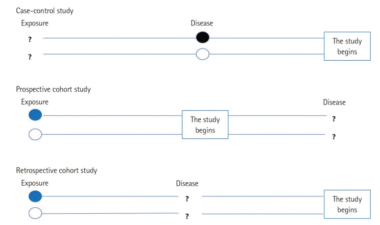
| Case-control | Outcome → Exposure (retrospective) | Odds ratio | Rare diseases, multiple exposures |
| Prospective cohort | Exposure → Outcome (forward) | Relative risk, incidence | Rare exposures, multiple outcomes |
| Retrospective cohort | Historical exposure → Outcome (backward) | Relative risk | Occupational exposures |
Case-control starts with people who have the disease and looks back for exposures. Efficient for rare diseases and long-latency outcomes (cancer, birth defects). Calculates odds ratios. Vulnerable to recall bias.
Cohort starts with exposure and follows forward to outcome. Allows direct calculation of incidence and RR. Efficient for rare exposures or studying multiple outcomes. Expensive and slow for rare outcomes.
Nested and Hybrid Designs
| Design | Description | Advantage |
|---|---|---|
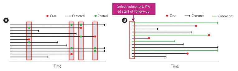
| Nested case-control | Cases and controls selected from within an established cohort | Retains cohort advantages, reduces cost |
| Case-cohort | Cases compared to a random subcohort sampled at baseline | One subcohort can serve multiple outcomes |
| Case-crossover | Each case serves as own control at a different time | Controls for fixed confounders (genetics, sex) |
| Ambidirectional cohort | Combines retrospective and prospective data | Combines historical and new data |
Advantages & Disadvantages Summary
| Design | Advantages | Disadvantages |
|---|---|---|
| Cross-sectional | Fast, inexpensive, measures prevalence | No temporality, cannot infer causation |
| Case-control | Efficient for rare diseases & long latency | Recall bias, selection of controls difficult |
| Cohort | Temporal sequence clear, multiple outcomes | Expensive, long duration, loss to follow-up |
| RCT | Best for causation, controls confounders | Expensive, ethical limits, artificial populations |
23 Randomized Controlled Trials & Phases
The randomized controlled trial is the gold standard for establishing causation and evaluating interventions. Random allocation controls for both known and unknown confounders, allowing causal inference.
Key Features of RCTs
- Randomization: Allocation by chance eliminates selection bias and distributes confounders equally
- Allocation concealment: Those enrolling patients cannot know or predict the next assignment
- Blinding: Single-blind (patient only), double-blind (patient + investigator), triple-blind (+ analyst)
- Control group: Placebo or active comparator
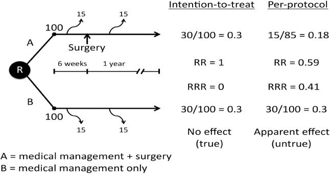
- Intention-to-treat (ITT) analysis: Patients analyzed in their assigned group regardless of adherence — preserves randomization
- Per-protocol analysis: Only patients who completed assigned treatment — can introduce bias
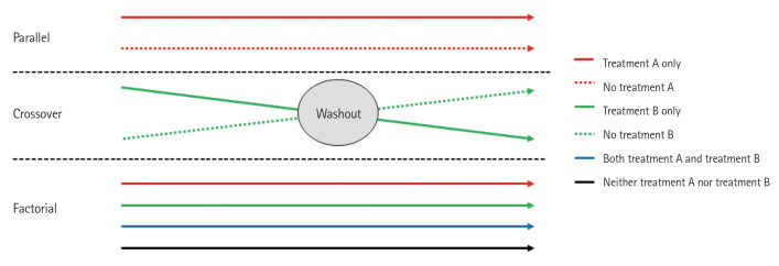
RCT Variants
| Design | Description |
|---|---|
| Parallel group | Each subject receives one treatment for the study duration |
| Crossover | Each subject receives both treatments sequentially (self-control) |
| Factorial | Simultaneously tests ≥2 interventions (e.g., 2×2 factorial) |
| Cluster randomized | Groups (clinics, villages) randomized rather than individuals |
| Adaptive | Design modified based on accumulating data (e.g., dropping dose arms) |
| Pragmatic | Tests effectiveness under real-world conditions |
| Explanatory | Tests efficacy under ideal conditions |
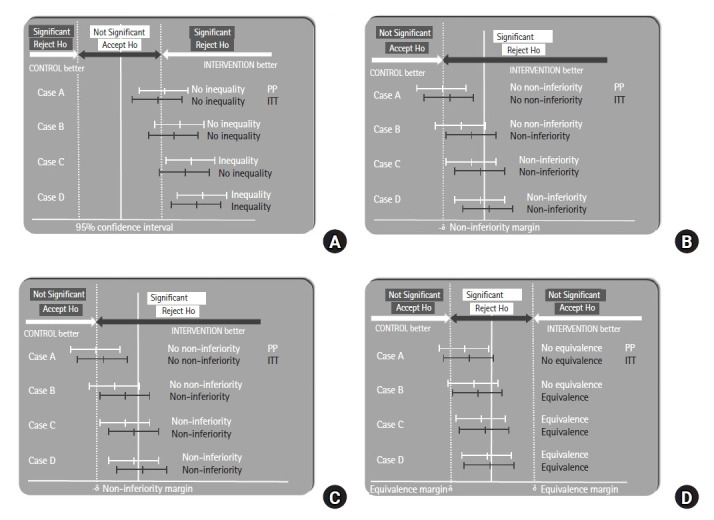
| Non-inferiority | Tests whether new treatment is not worse than standard by a margin |
| Equivalence | Tests whether two treatments are essentially the same |
Clinical Trial Phases
| Phase | Purpose | Subjects | Size |
|---|---|---|---|
| Phase 0 | Microdosing PK in humans (optional) | Healthy volunteers | ~10 |
| Phase I | Safety, MTD, PK | Healthy volunteers | 20–80 |
| Phase II | Efficacy, dosing, side effects | Patients | 100–300 |
| Phase III | Confirmatory efficacy vs standard | Patients | 1,000–3,000 |
| Phase IV | Post-marketing surveillance | General population | Thousands+ |
Randomization Methods
| Method | Description |
|---|---|
| Simple randomization | Coin flip or random number generator per subject |
| Block randomization | Groups of fixed size randomized to ensure balance |
| Stratified randomization | Separate randomization within baseline strata (e.g., age, sex) |
| Minimization | Dynamic allocation to balance multiple factors |
| Cluster randomization | Randomize groups (clinics, schools) instead of individuals |
Bias Prevention in RCTs
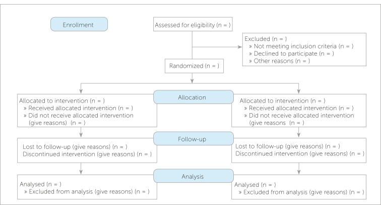
The CONSORT (Consolidated Standards of Reporting Trials) guidelines mandate transparent reporting of randomization, allocation concealment, blinding, primary and secondary outcomes, and loss to follow-up. Risk of bias tools (e.g., Cochrane Risk of Bias 2) systematically assess each domain. Trials with unconcealed allocation or inadequate blinding consistently overestimate treatment effects compared to rigorously conducted trials.
24 Meta-Analysis, Systematic Review & GRADE
Systematic reviews and meta-analyses synthesize evidence across multiple studies to produce more precise estimates and resolve conflicting findings. They sit at the top of the evidence hierarchy when well-conducted.
Systematic Review vs Meta-Analysis
- Systematic review: Structured, comprehensive, reproducible synthesis of all relevant literature on a question using predefined criteria.
- Meta-analysis: Statistical combination of results from multiple studies to produce a pooled effect estimate.
- Every meta-analysis should be based on a systematic review; not every systematic review yields a meta-analysis.
Key Concepts in Meta-Analysis
| Concept | Description |
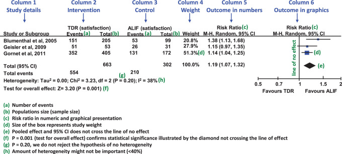
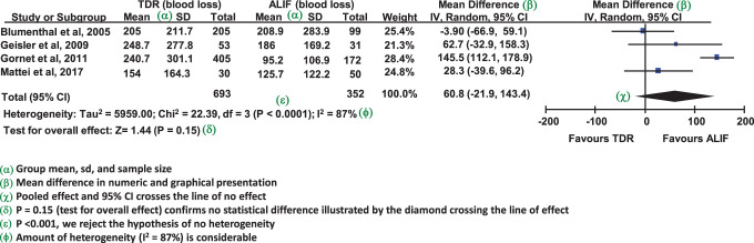
|---|---|
| Forest plot | Graphical display of individual study effects, CIs, and pooled estimate |
| Heterogeneity (I²) | Variability in effect sizes across studies; > 50% is substantial |
| Fixed-effect model | Assumes single true effect across studies |
| Random-effects model | Assumes true effects vary across studies |
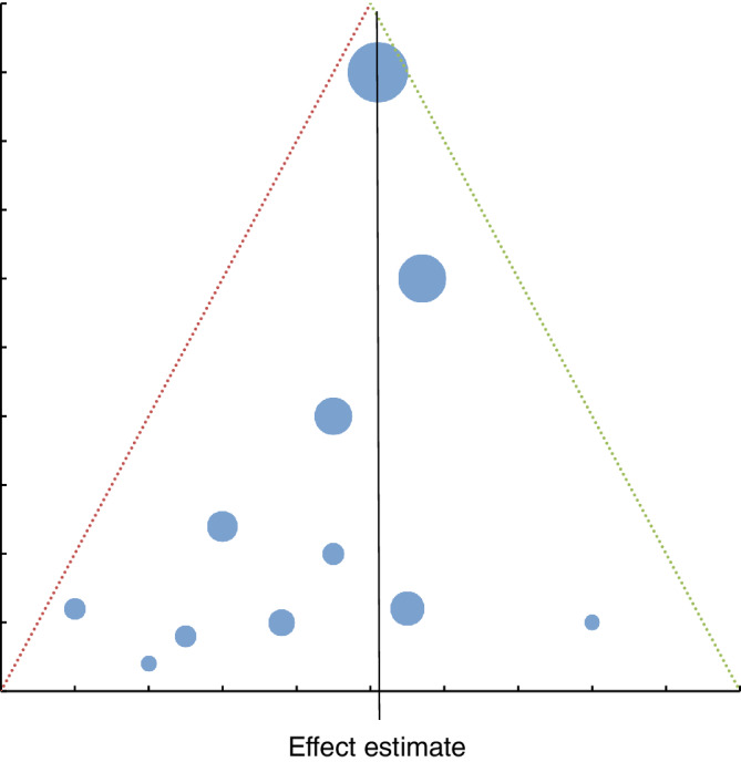
| Funnel plot | Detects publication bias (asymmetry suggests missing small negative studies) |
| Egger test | Statistical test for funnel plot asymmetry |
GRADE Framework
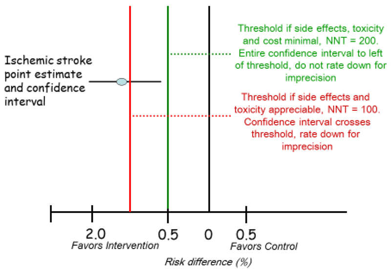
The Grading of Recommendations Assessment, Development and Evaluation (GRADE) framework rates the quality of evidence (high, moderate, low, very low) and strength of recommendations (strong or weak/conditional). RCTs start at high quality and can be downgraded for risk of bias, inconsistency, indirectness, imprecision, and publication bias. Observational studies start at low quality and can be upgraded for large effects, dose-response, or plausible confounding that would bias toward null.
PRISMA & Reporting Standards
The PRISMA (Preferred Reporting Items for Systematic reviews and Meta-Analyses) statement provides a checklist for transparent reporting. Other reporting standards include CONSORT for RCTs, STROBE for observational studies, STARD for diagnostic accuracy studies, and TRIPOD for prediction model studies. Familiarity with these standards is valuable both for authors writing papers and for readers critiquing them.
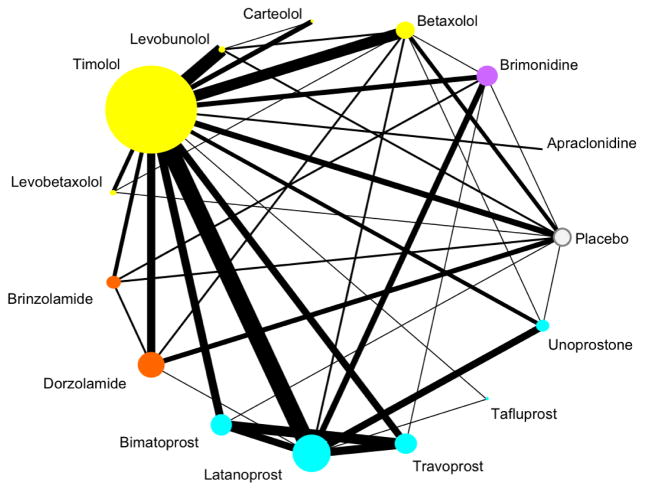
Network Meta-Analysis
When several treatments have been compared to various controls in different trials, a network meta-analysis combines direct (head-to-head) and indirect (via common comparator) evidence to rank treatments and estimate comparative effects that were never directly tested. This methodology is increasingly important for guideline development when multiple competing therapies exist.
25 Bias & Error Types
Bias is systematic error that distorts study results in a particular direction. Unlike random error, bias cannot be fixed by increasing sample size — it must be prevented through careful study design.
Selection Bias
| Type | Description | Prevention |
|---|---|---|
| Sampling (ascertainment) | Sample not representative of population | Random sampling |
| Berkson bias | Hospital-based controls differ from community | Use community controls |
| Neyman (prevalence-incidence) | Missing cases who died or recovered before sampling | Use incident cases |
| Healthy worker effect | Workers healthier than general population | Use worker comparison group |
| Attrition bias | Differential loss to follow-up between groups | Minimize loss; ITT analysis |
| Non-response bias | Responders differ from non-responders | Maximize response rate |
Information (Measurement) Bias
| Type | Description | Example |
|---|---|---|
| Recall bias | Diseased recall exposures differently | Mothers of malformed infants recall drugs more |
| Interviewer/observer bias | Interviewer probes one group more | Knowing case status affects history-taking |
| Hawthorne effect | Subjects change behavior when observed | Better medication adherence when monitored |
| Misclassification | Errors in assigning exposure or outcome | Imperfect diagnostic criteria |
| Publication bias | Positive results more likely to be published | Missing "negative" trials skews literature |
Time-Related Biases
| Bias | Description |
|---|---|
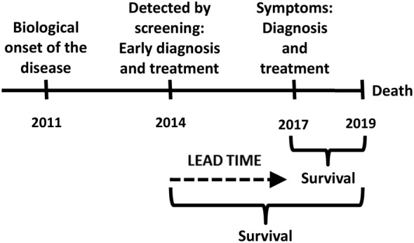
| Lead-time bias | Screening detects disease earlier; apparent longer survival without true benefit |
| Length-time bias | Screening preferentially detects slowly progressive cases |
| Immortal time bias | Time window during which outcome cannot occur misclassified |
| Survivor bias | Only survivors available for study; dead patients excluded |
Random vs Systematic Error
| Feature | Random Error | Systematic Error (Bias) |
|---|---|---|
| Source | Chance variation in sampling or measurement | Flaws in study design or execution |
| Effect on validity | Reduces precision | Distorts accuracy |
| Effect on CI | Wider intervals | Shifted point estimate |
| Fix | Larger sample size | Better design; cannot be fixed by more data |
Detection & Control of Bias
Bias cannot be eliminated entirely, but its influence can be minimized through careful study design, strict protocols, and thoughtful analysis. Sensitivity analyses can test how robust conclusions are to plausible biases. External validation of findings in independent populations remains one of the most powerful tools for confirming that a result is not an artifact of bias in the original study.
26 Confounding, Effect Modification & Causation
Confounding
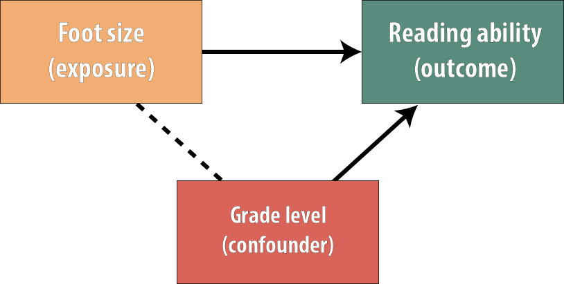
A confounder is a variable that is (1) associated with the exposure, (2) independently associated with the outcome, and (3) not on the causal pathway between exposure and outcome. Confounding distorts the apparent relationship between exposure and outcome.
Methods to Control Confounding
| Stage | Method | Description |
|---|---|---|
| Design | Randomization | Distributes known & unknown confounders equally |
| Restriction | Limit study to one value of confounder | |
| Matching | Pair exposed/unexposed on confounder | |
| Analysis | Stratification | Analyze within levels of confounder (Mantel-Haenszel) |
| Multivariable adjustment | Include confounders in regression model | |
| Propensity scores | Match or adjust on probability of exposure |
Effect Modification (Interaction)
Effect modification occurs when the effect of exposure on outcome differs across strata of a third variable. Unlike confounding, which is a nuisance to be controlled, effect modification is a biological or clinical finding to be reported. For example, aspirin reduces cardiovascular events more in men than in women — sex is an effect modifier, not a confounder.
Internal vs External Validity
- Internal validity: Extent to which study findings accurately reflect the true relationship in the study population. Threatened by bias, confounding, chance.
- External validity (generalizability): Extent to which findings apply to other populations, settings, or conditions. Threatened by restrictive inclusion criteria, artificial settings.
Hill Criteria for Causation
Sir Austin Bradford Hill's 1965 criteria remain the standard framework for inferring causation from observational data:
- Strength of association (larger RR more likely causal)
- Consistency across studies and populations
- Specificity of association (one cause, one effect)
- Temporality (cause precedes effect) — only absolute requirement
- Biological gradient (dose-response)
- Plausibility (biological mechanism)
- Coherence with existing knowledge
- Experiment (intervention supports effect)
- Analogy (similar causes produce similar effects)
Ecologic fallacy: Inferring individual-level relationships from group-level data (e.g., countries with more TVs have lower infant mortality does not mean TVs prevent infant death).
Reverse causation: Mistaking effect for cause. Depression correlates with cancer, but early cancer may cause depression rather than vice versa. Prospective studies establishing temporality are essential.
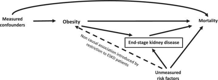
Example: Confounding by Indication
A particularly challenging form of confounding in pharmacoepidemiology is confounding by indication, where the reason a drug was prescribed (disease severity, comorbidities) is itself associated with the outcome. Observational studies of antibiotic use and mortality are often confounded this way: sicker patients are more likely to receive antibiotics and more likely to die, making antibiotics appear harmful when they are not. This is one reason RCTs are essential for evaluating therapies.
Detecting Effect Modification
Effect modification is assessed by testing for statistical interaction — adding an interaction term (exposure × modifier) to a regression model. A significant interaction suggests the exposure effect differs across levels of the modifier. Effect modification should be reported, not eliminated. Stratum-specific estimates are the primary output, not pooled summary measures.
27 Screening & USPSTF Principles
Screening is the testing of asymptomatic individuals to detect disease at an earlier, more treatable stage. Effective screening requires meeting specific criteria to justify its cost, harms, and population impact.
WHO / Wilson-Jungner Criteria for Screening
- Disease is an important health problem
- Natural history of disease is understood
- Recognizable early or latent stage exists
- Suitable screening test available (sensitive, acceptable, affordable)
- Effective treatment available for early-stage disease
- Treatment at early stage improves outcomes vs later treatment
- Facilities for diagnosis and treatment are available
- Cost-effective relative to health benefit
- Continuous process, not one-time effort
USPSTF Recommendation Grades
| Grade | Meaning | Suggested Practice |
|---|---|---|
| A | High certainty of substantial net benefit | Offer the service |
| B | Moderate/high certainty of moderate net benefit | Offer the service |
| C | Small net benefit; individualize | Offer selectively |
| D | No net benefit or harms outweigh benefits | Discourage |
| I | Insufficient evidence | Clinical judgment |
Major USPSTF Grade A & B Recommendations
| Screening | Population | Grade |
|---|---|---|
| Colorectal cancer | Adults 45–75 | A/B |
| Mammography | Women 50–74 (biennial) | B |
| Cervical cancer (Pap) | Women 21–65 | A |
| Lung cancer (LDCT) | Adults 50–80 with smoking history | B |
| Abdominal aortic aneurysm | Men 65–75 who ever smoked | B |
| Hypertension | Adults ≥18 | A |
| HIV | Adolescents & adults 15–65 | A |
| Hepatitis C | Adults 18–79 | B |
| Type 2 diabetes | Adults 35–70 with overweight/obesity | B |
Overdiagnosis
Overdiagnosis is the detection of disease that would never have caused symptoms or death during the patient's lifetime. It differs from misdiagnosis (wrong diagnosis) in that the pathology is real but indolent. Overdiagnosis is particularly common in cancers with highly variable biology (prostate, thyroid, early breast, indolent lung lesions). Every overdiagnosed patient is exposed to treatment harms without possibility of benefit.
28 High-Yield Review
The following is a distilled review of the most commonly tested and clinically essential concepts in biostatistics and epidemiology.
Statistical Test Selection Cheat Sheet
| Outcome | Groups | Parametric | Non-Parametric |
|---|---|---|---|
| Continuous | 1 sample vs known | One-sample t-test | Wilcoxon signed-rank |
| Continuous | 2 independent | Independent t-test | Mann-Whitney U |
| Continuous | 2 paired | Paired t-test | Wilcoxon signed-rank |
| Continuous | ≥3 independent | One-way ANOVA | Kruskal-Wallis |
| Continuous | ≥3 paired | Repeated-measures ANOVA | Friedman |
| Categorical | 2+ independent | — | Chi-square / Fisher |
| Categorical | Paired binary | — | McNemar |
| Time-to-event | 2+ groups | — | Log-rank / Cox |
| Association 2 continuous | — | Pearson | Spearman |
Top 20 Concepts to Master
- Sensitivity, specificity, PPV, NPV and the effect of prevalence
- Likelihood ratios and Bayesian updating of pre-test probability
- Relative risk, odds ratio, absolute risk reduction, NNT
- Confidence intervals: interpretation and construction
- p-values: definition and common misinterpretations
- Type I/II errors and statistical power
- Central limit theorem and sampling distributions
- Normal distribution properties (68-95-99.7 rule)
- Mean, median, mode in symmetric vs skewed data
- Standard deviation vs standard error
- Choosing parametric vs non-parametric tests
- Chi-square and Fisher exact for categorical data
- Kaplan-Meier survival curves and log-rank test
- Cohort vs case-control vs cross-sectional designs
- RCT features: randomization, blinding, ITT analysis
- Systematic review and meta-analysis (forest plot, I²)
- Bias types: selection, information, lead-time, length-time
- Confounding vs effect modification
- Hill criteria for causation
- USPSTF grades and screening principles
Must-Know Formulas
| Measure | Formula |
|---|---|
| Sensitivity | TP / (TP + FN) |
| Specificity | TN / (TN + FP) |
| PPV | TP / (TP + FP) |
| NPV | TN / (TN + FN) |
| LR+ | SN / (1 − SP) |
| LR− | (1 − SN) / SP |
| Relative risk | [a/(a+b)] / [c/(c+d)] |
| Odds ratio | (a×d) / (b×c) |
| ARR | Riskcontrol − Risktreatment |
| NNT | 1 / ARR |
| Attributable risk | Riskexposed − Riskunexposed |
| 95% CI (mean) | x̄ ± 1.96 × SE |
| SE of mean | s / √n |
Study Design Quick Reference
| Question | Best Design |
|---|---|
| Does treatment X work? | RCT |
| What causes rare disease Y? | Case-control |
| What is the risk of rare exposure Z? | Cohort |
| How common is disease W? | Cross-sectional (prevalence) |
| Does screening save lives? | RCT with mortality endpoint |
| Synthesizing existing evidence | Systematic review / meta-analysis |
| Outbreak investigation | Case-control or retrospective cohort |
Common Pitfalls & Misinterpretations
- p < 0.05 does not mean clinically important. Always evaluate effect size and CI.
- Non-significant does not mean no effect. Check power and CI width.
- Correlation does not equal causation. Consider confounding and reverse causation.
- RR and OR are not identical. OR overestimates RR when disease is common.
- PPV depends on prevalence. High specificity is not enough in low-prevalence screening.
- Lead-time bias makes screened patients appear to live longer even without benefit.
- ITT preserves randomization. Per-protocol analysis introduces bias.
- Confidence intervals beat p-values because they convey both direction and precision.
- Funnel plot asymmetry suggests publication bias in meta-analyses.
- Ecologic fallacy — group-level data cannot be used to infer individual-level relationships.
Key Rules of Thumb
- n ≥ 30 is usually large enough for the central limit theorem to apply
- Expected cell counts ≥ 5 are needed for chi-square; otherwise use Fisher exact
- Power ≥ 80% is the conventional minimum for trial design
- I² > 50% suggests substantial heterogeneity in meta-analysis
- LR+ > 10 and LR− < 0.1 are clinically useful thresholds
- κ > 0.6 indicates substantial inter-rater agreement
- AUC > 0.8 indicates good discrimination for a diagnostic test
- VIF > 5 suggests problematic multicollinearity
Landmark Trials & Studies
| Study | Contribution |
|---|---|
| Streptomycin TB trial (1948) | First modern RCT |
| Framingham Heart Study (1948–) | Identified cardiovascular risk factors; pioneered cohort methods |
| Doll & Hill British Doctors Study | Established smoking-lung cancer causation |
| UGDP (1970) | First trial to raise drug-safety concerns (tolbutamide) |
| Women's Health Initiative (2002) | Overturned HRT benefits observed in cohort studies |
| ALLHAT (2002) | Thiazide diuretics as first-line antihypertensive |
| Cochrane Collaboration (1993–) | Popularized systematic review methodology |
High-Yield Epidemiology Pearls
- Incidence measures new cases; prevalence measures existing cases.
- Prevalence = Incidence × Duration (approximately, for stable conditions).
- A highly SeNsitive test rules disease OUT; a highly SPecific test rules disease IN.
- Likelihood ratios are prevalence-independent and combine with pre-test odds via Bayes.
- LR+ > 10 or LR− < 0.1 are clinically powerful.
- Randomization controls for both known and unknown confounders.
- Blinding prevents ascertainment and measurement bias, not selection bias.
- Hill criteria: temporality is the only absolute requirement for causation.
- Overdiagnosis is the most underappreciated harm of modern cancer screening.
- NNT is the most clinically intuitive measure of treatment benefit.
- Case-control studies yield odds ratios; cohort studies yield relative risks.
- Confidence intervals crossing 1.0 (for ratios) or 0 (for differences) are not significant.
- p-values do not measure effect size or clinical importance.
- Loss to follow-up > 20% threatens internal validity of cohort studies.
- Confounding is a property of the data; effect modification is a biological finding.
Critical Appraisal Framework
When reading a clinical research paper, apply a structured checklist:
- Research question: What was the PICO (population, intervention, comparison, outcome)?
- Study design: Is the design appropriate for the question?
- Internal validity: Was randomization adequate? Were patients blinded? Was ITT used? What was loss to follow-up?
- Results: What is the effect size? Is it statistically and clinically significant? What is the precision (CI width)?
- External validity: Do the patients resemble mine? Was the intervention feasible?
- Harms: What adverse effects were reported? How do benefits compare to harms (NNT vs NNH)?
- Conflicts of interest: Funding source? Author disclosures?
Common Board Exam Questions
| Stem Clue | Likely Answer |
|---|---|
| Study of rare disease with many exposures | Case-control |
| Measures incidence and multiple outcomes | Cohort |
| Measures prevalence at a point in time | Cross-sectional |
| Tests causation with randomization | RCT |
| Compares SN/SP to prevalence-dependent PPV | Bayesian reasoning / prevalence effect |
| Screening test detects earlier without saving lives | Lead-time bias |
| Mothers of sick infants recall exposures better | Recall bias |
| Mean = median = mode | Normal distribution |
| Mean > median > mode | Positive (right) skew |
| 2 groups, continuous outcome, normal | Independent t-test |
| 3+ groups, continuous outcome | ANOVA |
| Categorical 2×2, small sample | Fisher exact |
| Time-to-event with censoring | Kaplan-Meier / Cox |
Clinical Epidemiology Tools
| Tool | Purpose |
|---|---|
| Framingham Risk Score | 10-year cardiovascular risk estimation |
| ASCVD Risk Calculator | Pooled cohort equations for CV risk |
| CHA2DS2-VASc | Stroke risk in atrial fibrillation |
| HAS-BLED | Bleeding risk on anticoagulation |
| Wells score | Probability of PE or DVT |
| CURB-65 / PSI | Severity and mortality in pneumonia |
| MELD | Mortality in end-stage liver disease |
| APACHE II | ICU mortality risk |
| FRAX | 10-year fracture risk |
| Gail model | Breast cancer risk |
These clinical prediction rules apply biostatistical models at the bedside, transforming risk factor data into actionable probability estimates. Their development and validation illustrate the integration of epidemiology with clinical decision-making.
Biostatistics and epidemiology are not obstacles to clinical practice — they are its quantitative backbone. Every clinical decision involves implicit estimation of probabilities, weighing of benefits and harms, and inference from imperfect evidence. Physicians who internalize these tools become better diagnosticians, better interpreters of literature, and better advocates for their patients. The goal is not statistical expertise for its own sake but the capacity to reason carefully under uncertainty — the defining challenge of clinical medicine.
Mastery of biostatistics and epidemiology also enables participation in medicine's ongoing self-correction. Every generation of physicians inherits an evidence base built on the methodological insights of those who came before, and each generation is responsible for refining that base further. The principles in this reference — study design, inference, bias, causation — are the tools by which medical knowledge advances. Learning them well is part of the professional obligation of every clinician.